A spiking neuron made of qubits

Three trains of input spikes arrive at a neuron through its dendrites and one train of output spikes leaves along its axon. Inside the neuron are three single-qubit circuits, each a row of rotation gates and delay gates. — The quantum leaky integrate-and-fire neuron. Each incoming spike becomes a rotation gate, and each gap between spikes becomes a delay in which the qubit is left alone. Figure 2 in the paper.

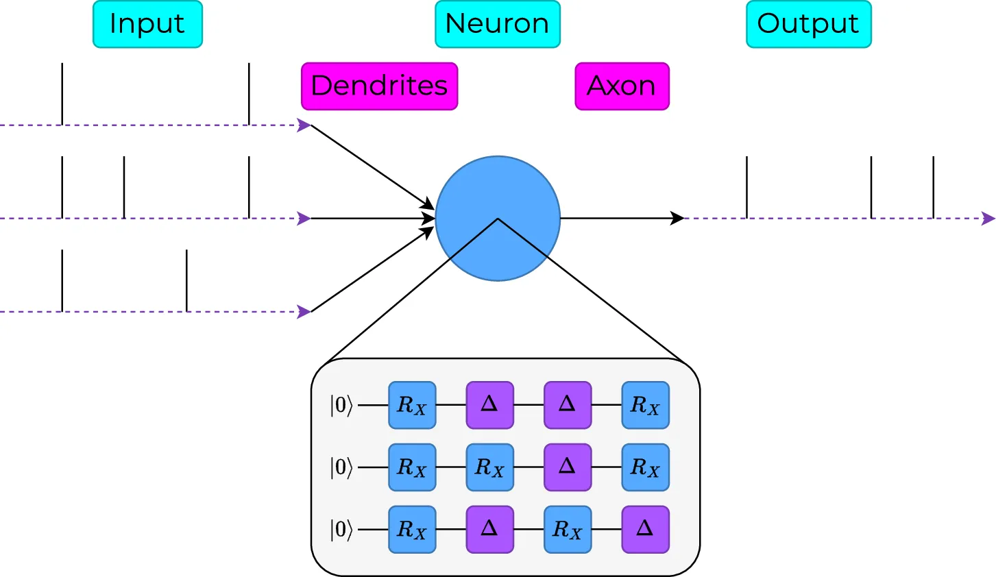
Two fields are trying to get past the limits of today’s computers. Quantum computing changes what the hardware is. Neuromorphic computing changes how it works, by copying the brain. Each has a problem the other can help with, and this paper is where I first put them together: a spiking neuron that runs on a quantum computer.

Two problems

The first problem is power. GPT-3 has 175 billion parameters and took an estimated 190 000 kWh to train. A human brain has about 100 billion neurons and runs on roughly 20 W. The comparison is rough, but the gap is too wide to blame on the details. Artificial neural networks keep the brain’s wiring diagram and throw away how neurons talk to each other.

Real neurons send short pulses, called spikes. A spike is all or nothing, so what carries information is when spikes arrive and how often. Spiking neural networks keep this. A neuron that receives nothing does nothing and costs nothing, and the timing of the spikes carries information that an ordinary network averages away.

The second problem belongs to quantum computing. Quantum machine learning mostly relies on variational circuits: long chains of gates whose settings are tuned until the circuit gives the right answers. Today’s quantum processors are noisy. A qubit holds its state for a short time, and every extra gate gives the noise another chance to spoil the result. The deeper the circuit, the worse this gets.

So I asked what the smallest useful quantum neuron would look like, and whether the noise could do some of the work.

The classical neuron

The leaky integrate-and-fire neuron dates from 1907 and is still the usual choice for spiking networks, because it is cheap to compute and close enough to biology to be useful. Its name lists what it does.

Integrate. Each incoming spike raises the neuron’s membrane potential.
Leak. With no input, the potential decays back towards zero.
Fire. When the potential crosses a threshold, the neuron sends a spike of its own and resets.

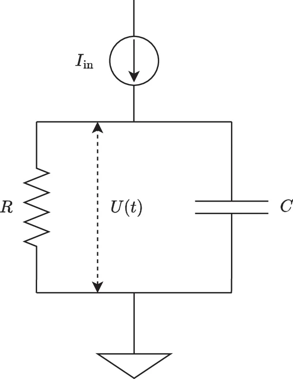
As electronics, this is a resistor and a capacitor side by side. Current charges the capacitor, the resistor drains it, and the voltage across them is the membrane potential.

A circuit diagram. An input current feeds a resistor and a capacitor wired in parallel, and the voltage across them is labelled as the membrane potential. — The classical neuron as a resistor and a capacitor. The capacitor integrates the input and the resistor leaks it away. Figure 1 in the paper.

The same neuron on one qubit

Each of the three behaviours has a natural partner on a quantum computer.

The membrane potential becomes the qubit’s excited-state population: the chance, between 0 and 1, of finding the qubit in its excited state when it is measured.

A spike becomes a rotation gate, R_X(θ). It turns the qubit away from its ground state and raises the population. The angle θ sets how hard the spike hits.

The leak costs nothing. An excited qubit that is left alone relaxes to its ground state, because it is never fully cut off from its surroundings. This is T₁ relaxation, and it is an exponential decay, which is the exact shape the neuron’s leak needs. When no spike arrives, the circuit waits for a time τ and the hardware supplies the leak.

Firing needs a measurement. After each time step the population is read out. If it is over the threshold, the neuron records an output spike and the qubit is reset.

Remembering without a long circuit

Measuring a qubit destroys its state, so after each readout the neuron has to be put back where it was before the next input arrives. The plain way to do that is to rebuild the whole history of gates at every step, and the circuit then grows without limit.

It does not have to. Every gate in the neuron is a rotation about the same axis, so any state the neuron can reach is one rotation away from the ground state. If the last measured population was α, a single gate with angle φ = 2 arcsin √α restores it. However long the neuron has been running, each step is the same short circuit: one gate for memory, then either a spike or a wait.

Two panels. The top panel shows four single-qubit circuits, one per time step, each one gate longer than the last. The bottom panel shows the compact form: a memory rotation gate, then an input gate, in a loop that repeats every time step. — Top: rebuilt from scratch, the circuit gains a gate at every time step. Bottom: what the neuron runs. One gate restores the last measured state and one handles the new input, however long it has been running. Figure 3 in the paper.

1qubit per neuron

2gates per time step, at most

0two-qubit gates, so the neurons never entangle

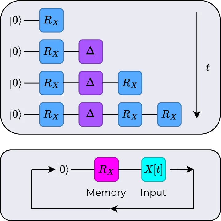
Because the neurons never entangle with each other, the cost of simulating them grows in step with their number, where a variational circuit’s cost grows much faster. The circuit is also too short for noise to build up in the way it does in a deep one.

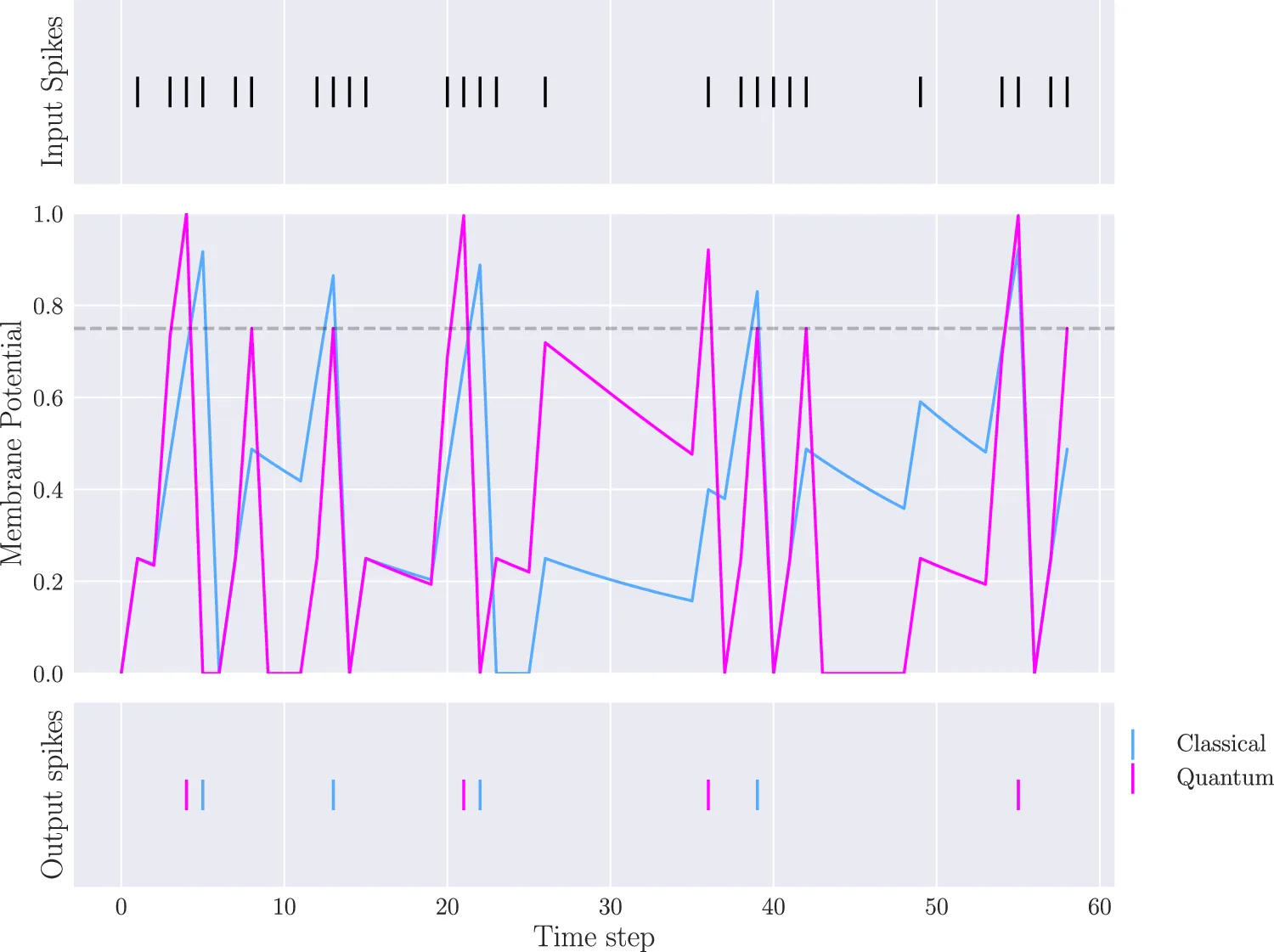
Fed the same train of random input spikes, the classical and quantum neurons behave alike. They rise on a spike, sag between spikes, and fire and reset at the threshold.

Three stacked plots over 60 time steps. The top shows random input spikes. The middle shows the classical membrane potential in blue and the quantum excited-state population in magenta, both rising with spikes, decaying between them, and resetting at a dashed threshold line at 0.75. The bottom shows the output spikes of each neuron. — The classical neuron (blue) and the quantum neuron (magenta) given the same input spikes. The dashed line is the firing threshold. Figure 4 in the paper.

From one neuron to a network

The quantum neuron drops into a network wherever a classical spiking neuron would go. An image is turned into spike trains, with brighter pixels spiking more often, and the spikes pass through the layers one time step at a time. At the output, the class whose neuron fires most is the answer.

One thing differs from the classical network. A classical connection has one weight to learn. Here each connection has two: the rotation angle θ, which sets how strongly a spike lands, and the delay τ, which sets how fast the neuron forgets. Both are trained together.

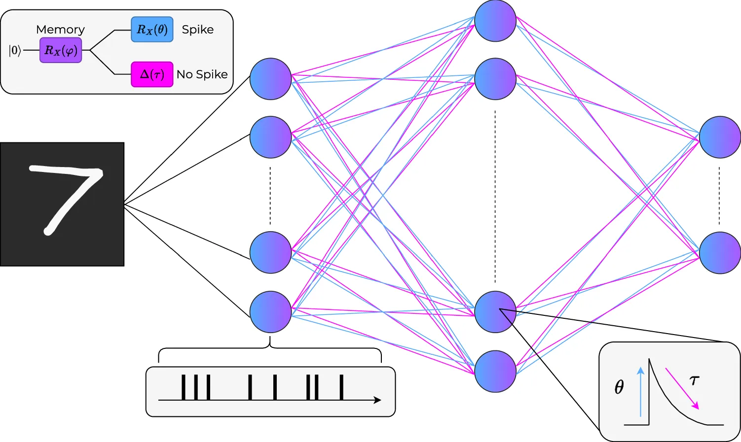
A fully connected network of three layers of neurons classifying a handwritten digit seven. Every connection is drawn twice, in blue for the rotation angle theta and in magenta for the delay tau. Insets show the input spike train, the neuron's circuit, and a spike that rises by theta and decays at a rate set by tau. — The quantum spiking neural network. Every connection carries two trained weights: θ in blue for spike strength and τ in magenta for the decay. Figure 5 in the paper.

Training uses backpropagation through time. A spike is a step, and a step has no usable gradient, so the backward pass swaps in a smooth stand-in for it. This is the standard fix for classical spiking networks and it carries over unchanged.

What we found

Francesco Petruccione and I built two versions, a fully connected network (QSNN) and a convolutional one (QSCNN). We tested them on three image sets: handwritten digits (MNIST), clothing (Fashion-MNIST) and handwritten Japanese characters (Kuzushiji-MNIST). We ran them against classical networks, classical spiking networks, and two established quantum models: a variational classifier (QNN) and a quanvolutional network (Quanv). Every model was kept small and as alike as we could make them, and all were trained on the same machine.

Model	MNIST	Fashion	Kuzushiji	Training time
ANN	97.84	87.24	90.38	30 s
SNN	95.84	81.73	90.02	2 m 26 s
QNN	89.65	82.90	67.18	54 m 22 s
Noisy QNN	86.82	80.68	59.18	5 h 27 m
QSNN	88.25	75.25	60.36	2 m 14 s
CNN	96.87	81.19	81.98	1 m 48 s
SCNN	97.75	65.81	82.06	5 m 49 s
Quanv	92.46	83.99	71.83	6 h 27 m
Noisy Quanv	92.35	82.87	70.58	31 h 26 m
QSCNN	90.62	70.19	66.02	5 m 40 s

Accuracy is the percentage correct on 10 000 test images. The quantum models were run as simulations on a classical computer.

The result is in the last column. On digits the spiking quantum networks score within a few points of the other quantum models, and they train in minutes where the others take hours.

Training time for all ten models. The axis is logarithmic, so each gridline is a step of six to ten times. Drawn from Table 1 of the paper.

24×faster than the variational network, without noise

146×faster once noise is simulated

333×faster for the convolutional version, with noise

Simulating noise costs the other quantum models hours of training and some of their accuracy. The spiking networks hardly change, because relaxation is already part of how they work.

Test accuracy of the six quantum models on the three image sets. The two spiking models are in bold. Drawn from Table 1 of the paper.

What it does not show

This is a proof of concept, and I would rather say where it stops than have a reader find out.

No quantum model here beats the classical networks. On these tasks an ordinary network is still the right tool.
On the two harder image sets the spiking quantum networks trail the other quantum models by several points. The networks were kept simple on purpose, and nothing was tuned to a dataset.
The numbers come from simulation. The design is meant for real noisy hardware, but running it there is later work.
Still images are a poor test of a spiking network. Its strength is data that unfolds in time.

What came next

The neuron has turned out to be a useful building block. I have since used it to classify EEG recordings of brain activity, which is data that really does unfold in time. With Donovan Slabbert I have used it as a kernel for spectral clustering. We have also gone the other way and derived a quantum neuron from the circuit equations of a memristive device, in place of building one from gates.

The code for every model in the table is on GitHub, written in Python with PyTorch.

The paper

A quantum leaky integrate-and-fire spiking neuron and network

Dean Brand, Francesco Petruccione

npj Quantum Information 10, 125 (2024)

Cite this paper

@article{brand2024qlif,
  title   = {A quantum leaky integrate-and-fire spiking neuron and network},
  author  = {Brand, Dean and Petruccione, Francesco},
  journal = {npj Quantum Information},
  volume  = {10},
  number  = {1},
  pages   = {125},
  year    = {2024},
  doi     = {10.1038/s41534-024-00921-x}
}

All research