Reading EEG with quantum neurons

The quantum spiking neuron was first tested on still images, which is a poor test of a spiking network. A photograph has no timing in it, so the timing has to be made up before the network can use it. This paper, written with Ravi Kumar Jha of Ulster University, gives the neuron data that is timed to begin with: recordings of a human brain.

Why brain signals

An EEG headset reads the voltage at a set of points on the scalp, many times a second. Each electrode gives a signal that rises and falls over time, and the electrodes sit at known places on the head. So the data has two kinds of structure at once. There is when something happened, and there is where. A signal in the brain travels, and the path it takes is part of what it means.

Most machine learning throws some of this away. The recording is flattened into a list of numbers, or cut into windows and averaged. That is one reason quantum machine learning has had little to say about neuroscience: its usual methods do not fit the shape of the data. A spiking network does. Its neurons already work in time, and if they are laid out in space to match the electrodes, the network keeps both.

The recordings

The data is a small set of recordings of one person moving their wrist: up, down, or held straight. It was recorded with an Emotiv headset and is shared with NeuCube, the network described below, so anyone can run the same test.

14electrodes on the scalp

128readings per second, for one second

60recordings: 20 of each movement

The 14 electrodes, seen from above with the nose at the top. Drawn from the electrode coordinates the model uses.

Sixty recordings is very little by the standards of machine learning. That is normal for brain data, which is slow and costly to collect, and it is one reason to want a model that can learn from few examples.

A network shaped like a brain

NeuCube is a spiking neural network made by Nikola Kasabov for this kind of data. We call it the cube. It works in four steps.

Turn the signal into spikes. Each electrode’s signal becomes a train of spikes.
Feed the spikes into the cube. The cube is 1 485 spiking neurons placed at three-dimensional brain coordinates. The input neurons sit where the electrodes are.
Let the cube learn without labels. As spikes pass through, a connection between two neurons grows stronger when the first fires just before the second, and weaker when the order is reversed. After training, the pattern of connections reflects how activity moved through the head.
Read the cube. How often each output neuron fired becomes a short list of numbers for each recording, and an ordinary classifier decides from those which movement it was.

The neurons in the cube are ordinarily classical leaky integrate-and-fire neurons. We replaced them with the quantum one.

Swapping in the quantum neuron

The quantum neuron is the one from the earlier paper, unchanged. A spike arriving is a rotation of a qubit. A gap between spikes is a delay, in which the qubit is left to relax. After each step the qubit is measured, and the neuron fires if its excited-state population has crossed a threshold.

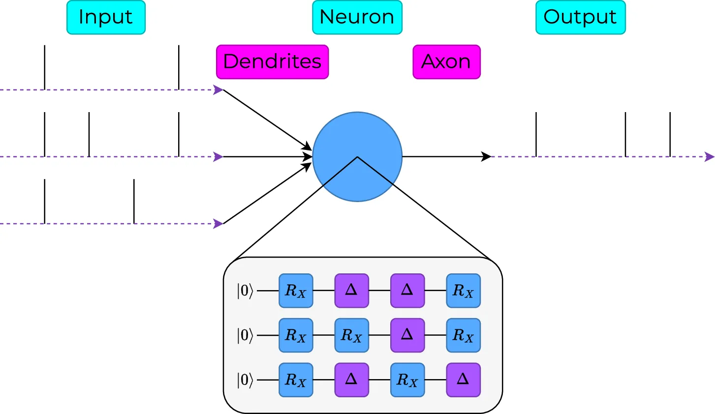
Three trains of input spikes arrive at a neuron through its dendrites and one train of output spikes leaves along its axon. Inside the neuron are three single-qubit circuits, each a row of rotation gates and delay gates. — The quantum leaky integrate-and-fire neuron. Each incoming spike becomes a rotation gate, and each gap between spikes becomes a delay in which the qubit is left alone. Figure 2 in the npj paper.

Because every gate is a rotation about one axis, the neuron’s whole history can be restored with a single gate after each measurement. Each step is at most two gates on one qubit, however long the recording.

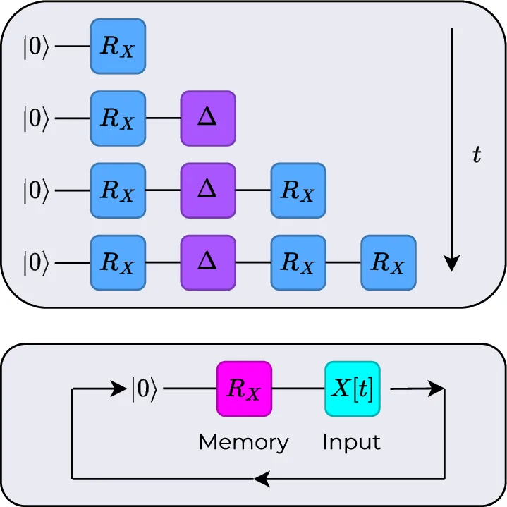
Two panels. The top panel shows four single-qubit circuits, one per time step, each one gate longer than the last. The bottom panel shows the compact form: a memory rotation gate, then an input gate, in a loop that repeats every time step. — Top: rebuilt from scratch, the circuit gains a gate at every time step. Bottom: what the neuron runs. One gate restores the last measured state and one handles the new input. Figure 3 in the npj paper.

The quantum neuron obeys the same kind of update rule as the classical one, so it needed no special handling. It went into the cube as a direct replacement, and the cube’s own learning rule worked on it as it stood.

The test

We built four models, so that each change could be judged alone.

Neurons alone. Fourteen neurons, one for each electrode, with no connections between them and no training. This shows what the neuron can do by itself.
Neurons in the cube. The full network, trained as described above.

Each was run twice, with classical neurons and with quantum neurons. Every setting the two kinds of neuron share was held the same.

The firing rates that came out were reduced to their two main components and handed to six standard classifiers, each scored by five-fold cross-validation. The task was always a choice between two movements, which gives three tasks. Two components is a severe cut. We made it so that a quantum classifier, which can only take a small input, can be put in that place later.

What we found

96%best accuracy with quantum neurons in the cube

82%best accuracy with classical neurons

Test accuracy averaged over the three tasks, for each classifier: naive Bayes (NB), linear discriminant analysis (LDA), decision tree (DT), random forest (RF), AdaBoost (AB) and support vector machine (SVM). Drawn from Figure 4 of the paper.

Three things stand out.

The tree-based classifiers are the ones to use. Decision tree, random forest and AdaBoost beat the other three for every model that uses the cube, so they are the fair place to compare.

The cube helps. With those classifiers, putting the neurons in a brain-shaped network beats using them alone. The data was recorded in three dimensions and is best handled in three dimensions.

The quantum neuron helps more. With a decision tree, quantum neurons in the cube are right 96% of the time and classical neurons in the cube 82%. With a decision tree or a random forest, the quantum neuron alone does better than the classical neuron with the whole cube behind it. The quantum cube’s results also vary less from one fold to the next. A second score, the Matthews correlation coefficient, gives the same ranking.

Quantum neurons in the cube come first on each of the three tasks, level with the quantum neuron alone on one of them.

Test accuracy with the decision tree classifier on each of the three two-way tasks. The movements are numbered as in the paper. Drawn from Figure 4 of the paper.

Why the quantum neuron might do better

The classical neuron applies its leak at every time step, whether or not a spike arrives, so its input and its decay are always mixed. The quantum neuron does one or the other: a spike rotates the qubit, and a gap lets it relax. Each of the two settings then controls one thing only, which makes the neuron’s behaviour easier to tune.

What it does not show

This is a proof of concept, not a benchmark. It is one person and sixty recordings, on a task the classical cube had already been shown to handle.
The quantum neurons were simulated on a classical computer. Nothing here says how they behave on noisy hardware.
The cube does not help with every classifier. With naive Bayes and linear discriminant analysis, both cube models fall to about 60% and the neurons alone do better.
The tasks were two-way choices. Telling all three movements apart at once is harder.

Where it leads

Nothing in the method depends on the data coming from a brain. Any signal with structure in both space and time will do, and financial forecasting is one we have in mind.

The next steps are larger and more varied datasets, runs on real noisy quantum hardware, and a quantum classifier in place of the classical one, so that the whole path from signal to answer is quantum.