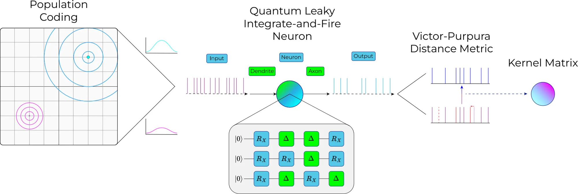
After the first paper on the quantum spiking neuron I went looking for other models it could be used in, and above all for ones where it could be set directly against established quantum algorithms. Kernel methods are the obvious case, since so much of quantum machine learning is built on them. Out of that came a spiking kernel: a way to measure how alike two data points are by the distance between the spike trains they produce. As far as we know it is new for classical spiking neurons as well as quantum ones. This paper, led by Donovan Slabbert and written with Francesco Petruccione, puts it to work in spectral clustering, against Donovan’s trainable quantum circuit kernel and a classical benchmark.
Clustering needs a sense of distance
Clustering sorts data into groups without being told what the groups are. The best-known method, K-means, looks for round clumps, and it fails on shapes that are not round: a ring inside a ring, or two interlocking crescents.
Spectral clustering handles those. It starts from a kernel matrix, a table that gives the similarity of every pair of points. It treats that table as a network, finds the few directions along which the network most naturally comes apart, and clusters the points in those directions, where a ring and its centre are easy to tell apart.
All of the skill is in the kernel. Give spectral clustering a good one and it will find the structure; give it a poor one and nothing downstream can rescue it. That makes the kernel a clean place to try something quantum, because nothing else in the method has to change. It is also a hard test. A quantum computer carries data into a very large space, and in that space the ordinary idea of distance often stops meaning much.
Two routes to a quantum kernel
The circuit route, which is Donovan’s. Each feature of a data point sets the angle of three rotations on a qubit, one about each axis, and each angle is scaled by a parameter. Two points are compared by how much their two quantum states overlap. The parameters are tuned so that the overlaps agree as well as they can with the known labels, and they are tuned by grid search, because gradients in circuits like this tend to vanish. The circuit has three rotations to a qubit and no entangling gates. That is deliberate. The spiking neuron works on one qubit at a time and entangles nothing, so the circuit was held to the same rule, and any difference between the two comes from how the kernel is built and not from one side having entanglement to draw on.
The spiking route, which is mine. No parameters are trained at all. Each point becomes a set of spike trains, the quantum neuron processes them, and two points are alike if the spike trains they produce are alike.
From a point to a train of spikes
A spiking neuron takes spikes, so the first job is to turn a position into spikes, and the two usual ways both fail here. Rate coding turns a larger number into more spikes. Temporal coding turns it into an earlier spike. For a brightness or a loudness that is sensible. For a coordinate it is wrong: a point far from the origin would shout, and a point near it would whisper, though neither matters more than the other.
The brain has the same problem and solves it with population coding. No single neuron reports the value. A whole row of neurons does, each with a value it prefers and a bell-shaped tuning curve around it. A neuron fires fast when the input is near its preferred value and slowly when it is far. The value is read from the pattern across the row.
For data with two features the row becomes a grid of receptive fields, as on the left of the figure at the top of this page. Every point in the dataset lights the grid in its own pattern, and points that lie close together light it alike. Each receptive field sends out a spike train, and each spike train goes through a quantum neuron.
The neuron in the middle
The neuron is the one from the first paper, unchanged. A spike rotates a qubit and raises its excited-state population. A gap lets the qubit relax, which is the leak. After each step the qubit is measured, and the neuron fires if the population has crossed a threshold. One more rotation restores the state after each measurement, so every step is two gates on one qubit, however long the train.
That matters more here than it did before. A kernel matrix needs every pair of points compared, so the work grows with the square of the dataset. A neuron that costs two gates and can be simulated in step with its size is one of the few quantum components cheap enough to use that way.
Comparing spike trains
What comes out is a set of spike trains for each data point. To fill in the kernel we need the distance between two spike trains, and neuroscience has two standard answers.
The van Rossum distance smooths each train, replacing every spike with a small decaying bump, and measures the gap between the two smooth curves. How long the bumps last sets how fussy it is about timing.
The Victor-Purpura distance is an edit distance, like the one a spell-checker uses. It is the lowest cost of turning one train into the other by adding spikes, deleting them, or sliding them in time. The price of a slide is the setting that matters. When sliding is cheap the distance only counts spikes. When it is dear, the distance cares whether spikes line up.
Either distance is turned into a similarity by a Gaussian, and the similarities are the kernel.
What we found
We tested on six datasets, with 300 points from each: three synthetic shapes (blobs, circles and moons), the Iris flower measurements with four features, and a catalogue of stars, galaxies and quasars from the Sloan Digital Sky Survey with ten features, in its natural proportions (SDSS) and in a balanced sample (SDSS*). After clustering, each cluster takes the label most common among its points, which lets us score accuracy against the true labels. We also scored the clustering itself with the adjusted Rand index, which is 1 for a perfect grouping and 0 for one no better than chance. Every figure below is the mean of six runs with different random seeds.
The quantum neuron keeps pace with the classical one. The two spiking kernels are nearly level everywhere, which is what a direct replacement should give. The quantum neuron is a little ahead on the moons and on Iris, the two datasets whose groups are most tangled, and a little behind on the blobs. This is one qubit and two gates, using neither superposition nor entanglement, and it matches a classical neuron built for the job.
Against the trainable circuit, the spiking kernel wins on shape. They are level on the blobs. On the circles the spiking kernel scores 0.96 on the Rand index and the circuit 0.50, and on the moons 0.55 against 0.34. These are the datasets where the groups curve round each other, and a kernel built from spike timing follows the curve better than overlaps between quantum states do.
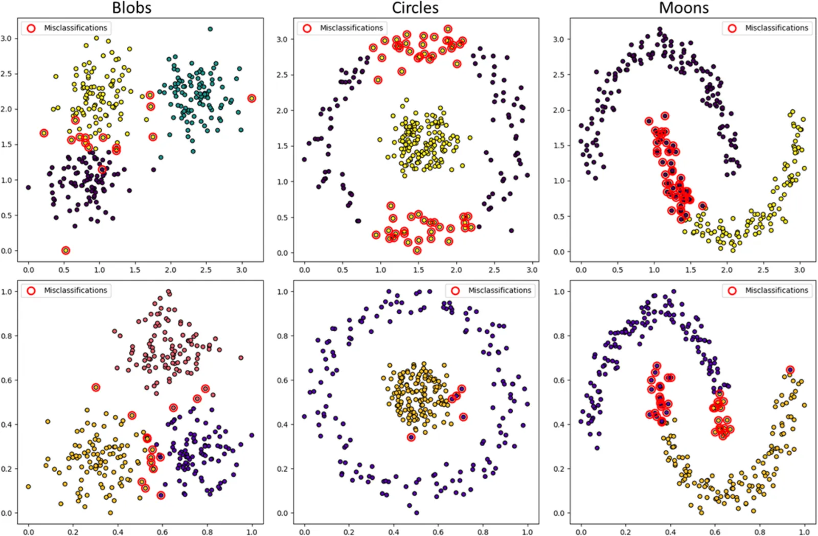
The choice of distance matters, and Victor-Purpura is the safe one. On the circles the van Rossum distance all but fails, while Victor-Purpura is close to perfect. It is not a clean sweep, since van Rossum does better on the moons. But Victor-Purpura never collapses, and it was faster to compute, so it is the only one we ran on the sky survey.
Where the spiking route breaks
On the sky survey the spiking kernels fail outright. Their Rand index is zero or very near it: the groups they find have nothing to do with stars, galaxies and quasars. The accuracy of 0.71 on the unbalanced data only reflects that one class is much the largest, and on the balanced data it drops to 0.40, which for three classes is close to guessing.
The cause is the encoding, not the neuron. A grid of receptive fields is cheap in two dimensions. In ten it is ruinous, because the number of grid cells multiplies with every feature added. To finish at all we had to make the grid coarse, and a coarse grid cannot tell the points apart. Even so, these runs took far longer than any of the others.
Reducing the data to fewer dimensions before encoding it would ease this. We did not, because the circuit was tested on all ten features and the comparison had to be like for like. We did try cutting both down to two dimensions, and every result got markedly worse.
The trainable circuit copes better here. It adds a qubit for each feature, not a grid dimension, and its parameters let it adapt to the data. It is still well short of good.
What it does not show
- Neither quantum kernel beats the classical one. The ordinary RBF kernel is ahead on nearly every dataset and nearly perfect on the four easier ones. For these problems it remains the right tool.
- The circuit was held to single-qubit gates to match the neuron. That makes the comparison fair, and it also means the spiking kernel beat a restricted circuit, not the best one that could be built. Nothing here is a claim of quantum advantage.
- The spiking results vary more from run to run than the circuit’s. The spike trains are drawn at random from the firing rates, and that randomness carries through the distance and the clustering. Six runs is few, and was what the computing time allowed.
- Accuracy here is second-hand. Clustering has no labels, so the labels are assigned afterwards by majority vote, and the accuracy says how good the grouping is, not how good a classifier would be.
- Only the kernel is quantum. The clustering that uses it is entirely classical.
- Everything was simulated. Running the full pipeline on hardware is out of reach for now, because a kernel matrix needs a circuit run for every pair of points. How either kernel behaves under real hardware noise is an open question.
- Each dataset was cut to 300 points, for the same reason.
Where it leads
The pipeline is modular: an encoding, a neuron, a distance. The neuron held up and the Victor-Purpura distance held up. The encoding is what failed, so that is where the work is. An encoding whose cost grows gently with the number of features, in place of a full grid, would let the spiking kernel be tried on the data that matter in practice.
Donovan’s side has its own next steps: more layers of gates, parameters that can turn a rotation backwards as well as forwards, and entangling layers, which the paper names as the natural extension for either route.